The principles involved in selecting the cheapest combination of variable factors can be seen in terms of a simple example. If a firm manufactures gold necklace chains in such a way that there are only two variable factors, labour (specifically, goldsmith-hours) and gold wire, the production function for such a firm will be y = f (x₁, x₂; k), in which the symbol k is included simply as a reminder that the number of chains producible by x₁ feet of gold wire and x₂ goldsmith-hours depends on the amount of machinery and other fixed capital available. Since there are only two variable factors, this production function can be portrayed graphically in a figure known as an isoquant diagram (Figure 1-->). In the graph, goldsmith-hours per month are plotted horizontally and the number of feet of gold wire used per month vertically. Each of the curved lines, called an isoquant, will then represent a certain number of necklace chains produced. The data displayed show that 100 goldsmith-hours plus 900 feet of gold wire can produce 200 necklace chains. But there are other combinations of variable inputs that could also produce 200 necklace chains per month. If the goldsmiths work more carefully and slowly, they can produce 200 chains from 850 feet of wire; but to produce so many chains more goldsmith-hours will be required, perhaps 130. The isoquant labelled “200” shows all the combinations of the variable inputs that will just suffice to produce 200 chains. The other two isoquants shown are interpreted similarly. It is obvious that many more isoquants, in principle an infinite number, could also be drawn. This diagram is a graphic display of the relationships expressed in the production function.

The cost data and the technological data can now be brought together. The variable cost of using x₁, x₂ units of the factors of production is written p₁x₁ + p₂x₂, and this information can be added to the isoquant diagram (Figure 2-->). The straight line labelled v₂, called the v₂-isocost line, shows all the combinations of input that can be purchased for a specified variable cost, v₂. The other two isocost lines shown are interpreted similarly. The general formula for an isocost line is p₁x₁ + p₂x₂ = v, in which v is some particular variable cost. The slope of an isocost line is found by dividing p₂ by p₁ and depends only on the ratio of the prices of the two factors.

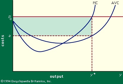The usual behaviour of average and marginal variable costs in response to changes in the level of output from a given fixed plant is shown in Figure 3-->. In this figure costs (in dollars per unit) are measured vertically and output (in units per year) is shown horizontally. The figure is drawn for some particular fixed plant, and it can be seen that average costs are fairly high for very low levels of output relative to the size of the plant, largely because there is not enough work to keep a well-balanced work force fully occupied. People are either idle much of the time or shifting, expensively, from job to job. As output increases from a low level, average costs decline to a low plateau. But as the capacity of the plant is approached, the inefficiencies incident on plant congestion force average costs up quite rapidly. Overtime may be incurred, outmoded equipment and inexperienced hands may be called into use, there may not be time to take machinery off the line for routine maintenance; or minor breakdowns and delays may disrupt schedules seriously because of inadequate slack and reserves. Thus the AVC curve has the flat-bottomed U-shape shown. The MC curve, as might be expected, falls faster and rises more rapidly than the AVC curve.

Such a conclusion is shown in Figure 3-->. In response to the price, p₀, shown, the firm will offer the quantity y* given by the value of y for which the ordinate of the MC curve equals the price. If a denotes the corresponding average variable cost, net revenue per unit will be equal to p₀ - a, and the total excess of revenues over variable costs will be y*(p₀ - a), which is represented graphically by the shaded rectangle in the figure.

The conclusion that marginal cost tends to equal price is important in that it shows how the quantity of output produced by a firm is influenced by the market price. If the market price is lower than the lowest point on the average variable cost curve, the firm will “cut its losses” by not producing anything. At any higher market price, the firm will produce the quantity for which marginal cost equals that price. Thus the quantity that the firm will produce in response to any price can be found in Figure 3--> by reading the marginal cost curve, and for this reason the marginal cost curve is said to be the short-run supply curve for the firm.

At any one time an established firm with an existing plant will make its short-run decisions by comparing the ruling price of its commodity with cost curves corresponding to that plant. If the price is so high that the firm is operating on the rising leg of its short-run cost curve, its marginal costs will be high—higher than its average costs—and it will be enjoying operating profits, as shown in Figure 3-->. The firm will then consider whether it could increase its profits by enlarging its plant. The effect of plant enlargement is to reduce the variable cost of producing high levels of output by reducing the strain on limited production facilities, at the expense of increasing the level of fixed costs.

Authoritative intermediate-level discussions may be found in William J. Baumol, Economic Theory and Operations Analysis, 4th ed. (1977). Vernon L. Smith, Investment and Production (1961), especially emphasizes the relationship between long-run costs and investment. Probably the best technical presentation is Paul A. Samuelson, Foundations of Economic Analysis, enlarged ed. (1983). George J. Stigler, Production and Distribution Theories (1941, reissued 1994), provides a discussion of the evolution of the theory. J. Viner, “Cost Curves and Supply Curves,” Zeitschrift für Nationalökonomie, 3:23–46 (1931), remains a classic text.Robert Dorfman Ed.